Note: While this tutorial shows how to implement hexagonal tiling in Unreal, the techniques presented below aren’t Unreal-specific and can be used in any shading language or node-based material system.

If you’re an artist working on games with vast environments, you’ve probably run into something like this at some point:

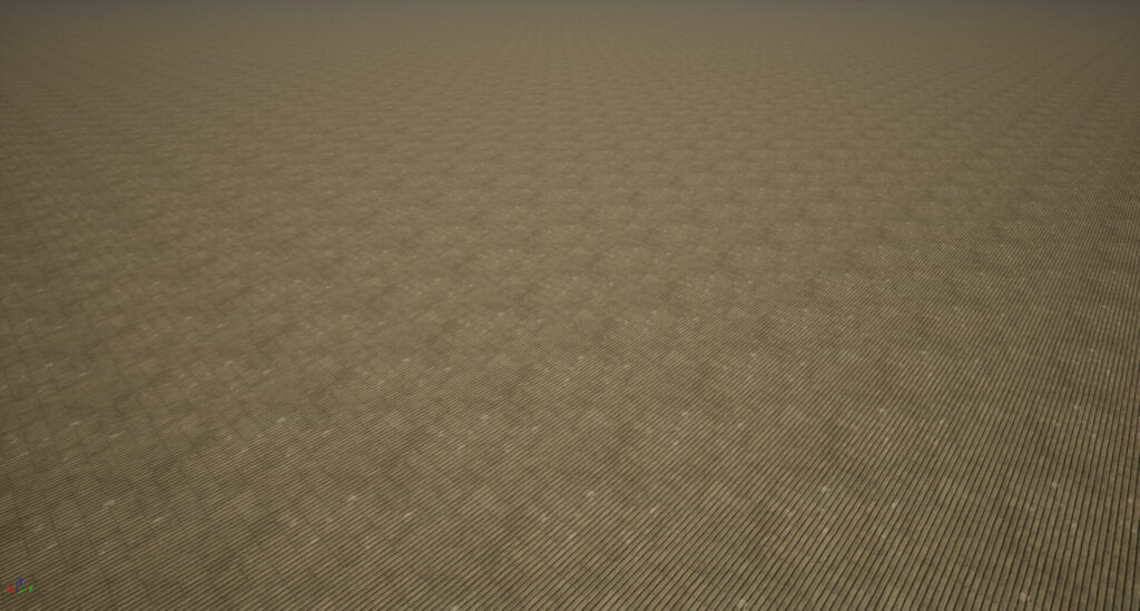
A texture covers a relatively small area, but is applied to a significantly larger surface, making it obvious that the texture is just repeated. There are ways to deal with this issue or at least make it less in-your-face:

• You can tweak the texture to make the repetition less obvious. Maybe paint out some unique details that only matter up close, or use a high pass filter to even out the brightness across the texture.
• Use detail maps to display textures with a different scale depending on the distance to the camera.
• Add additional details like decals or extra geometric details, to break up the surface and hide the repetition.

All these methods don’t really fix the underlying issue, there is still a grid-like repeating pattern, just not as noticeable. To really, truly get rid of it, you need to change how you’re mapping the texture.
So as a start, let’s rotate and offset the coordinates used in each 0.0-1.0 tile:

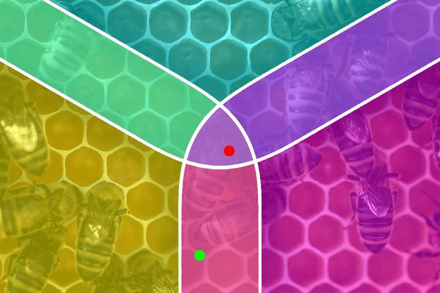
While the repetition has disappeared, the edges between the tiles are quite obvious. Can we improve this by blending between the individual tiles? Yes, but there is a drawback to this approach: Blending between the tiles necessitates multiple texture samples – specifically, four times, as there are four adjacent tiles at each corner.

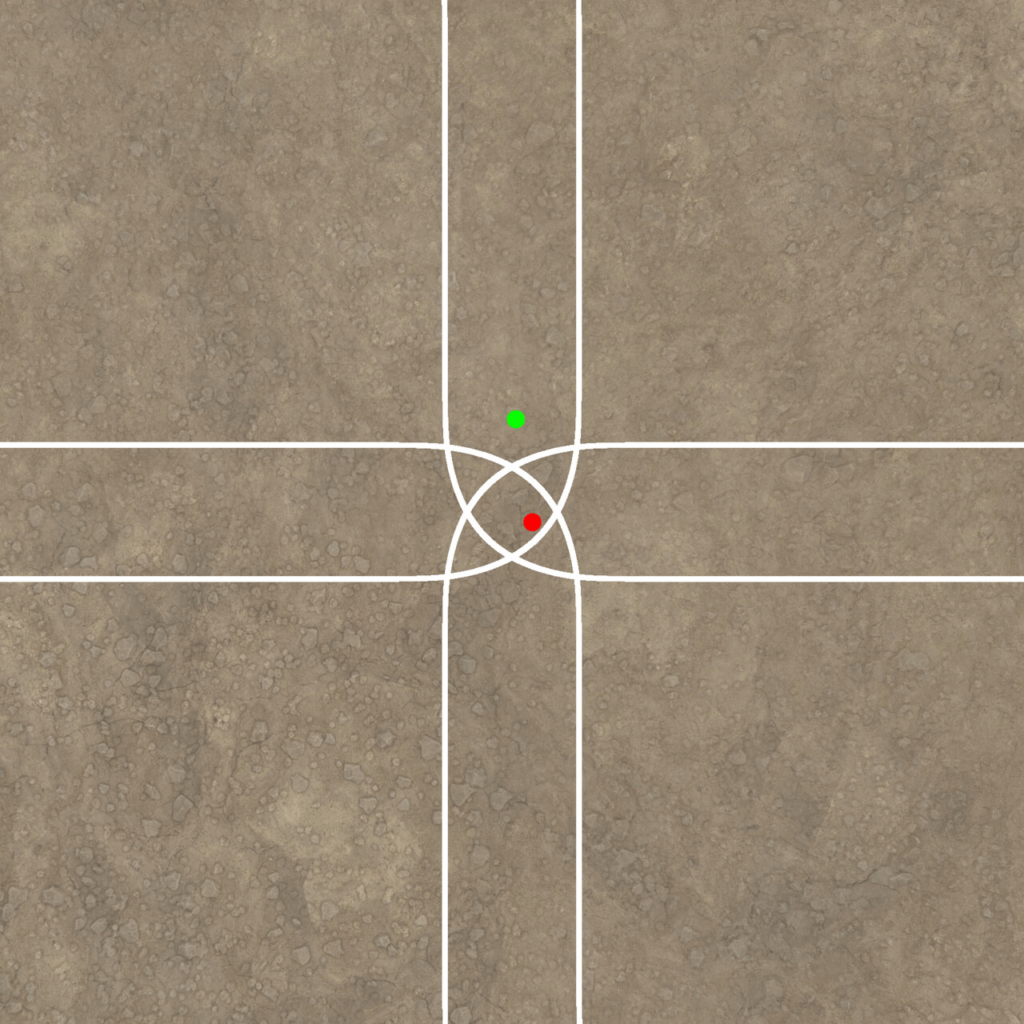
At the green dot, only two textures need to be sampled, but at the red dot, all 4 tiles are visible to some extent, so there is no way around sampling the texture 4 times. Surely there is a way to do this without affecting the performance that bad? Let’s see what happens when we use a hexagon instead of a square as tile format:

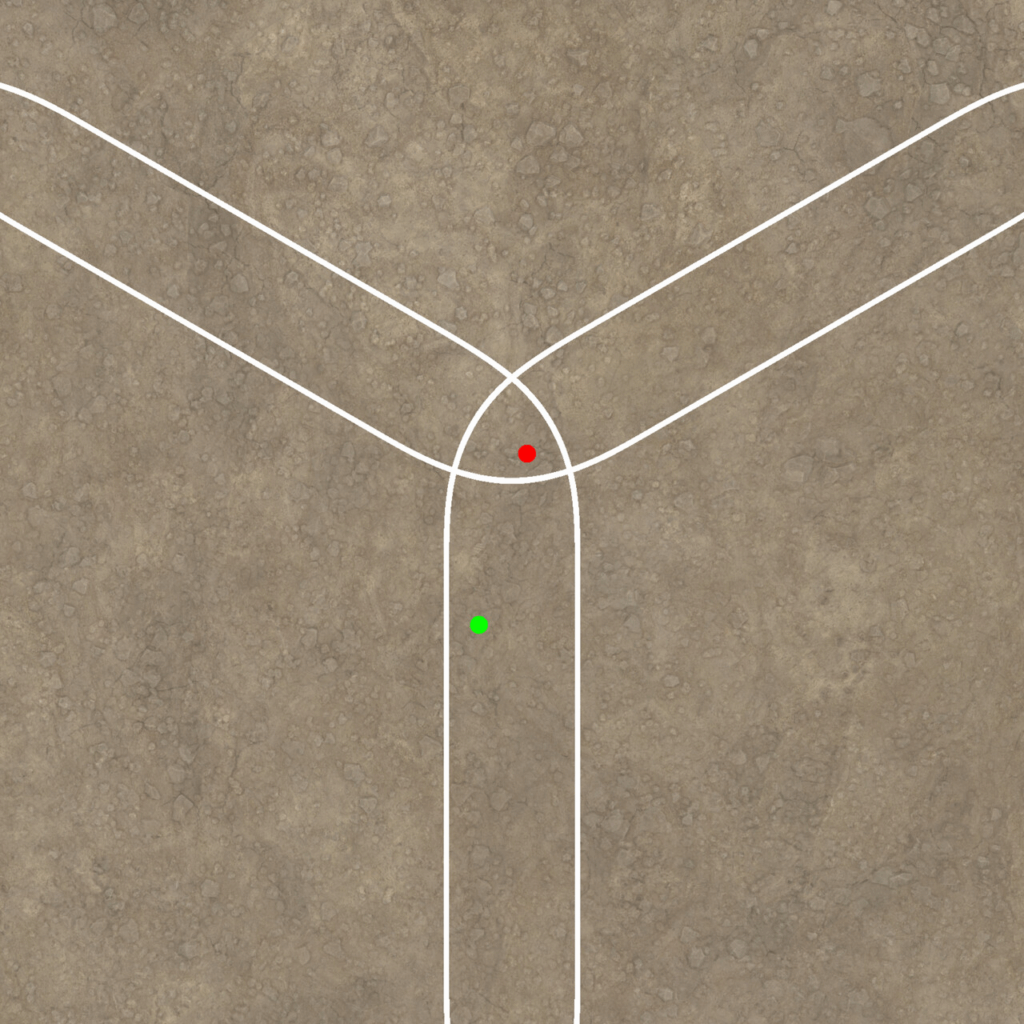
Now, we only have to sample 3 textures at most. Plus, the hexagon structure makes it more difficult to notice the pattern, since there are no straight, uninterrupted lines, making it more difficult for the viewer to spot the pattern.

Implementations

Hex tiling is a commonly used and well-tested technique. There are many great resources online on how to implement hex tiling:

• Ben Cloward made an in-depth video tutorial: https://youtu.be/F7UxUgow4yg
• When I tried out hex tiling, I used this paper by Thomas Deliot and Eric Heitz as reference: https://eheitzresearch.wordpress.com/738-2/ This implementation even employs histogram preservation to make sure that even with the texture blended multiple times, the contrast remains unaffected.
• There is also this implementation by Morten S. Mikkelsen that builds on the previous paper but doesn’t require additional precomputation steps: https://jcgt.org/published/0011/03/05/

All these implementations prioritize visual quality, and while they aren’t super expensive, the need to sample every texture three times instead of once wasn’t something I was super happy with. Landscape materials are notoriously complex, since they usually blend multiple layers of texture sets and incorporate various features like detail textures, noise overlays and modifications based on slopes or height.
So I wondered if I could make a cheaper version by sampling the texture only once, using dithering to hide the transitions.
While I’ll explain below how I implemented this, I want to emphasize that I don’t recommend this approach for every situation.
This method doesn’t reach the quality of proper blending. Using dithering instead of proper blending is always a compromise, and depending on your quality expectations, proper blending might be the way to go.

Dithering

Whenever you find yourself needing to sample a texture multiple times and blend the results, it’s worth considering whether you can achieve the same effect by blending the coordinates using dithering and then sampling the texture with the blended coordinates.

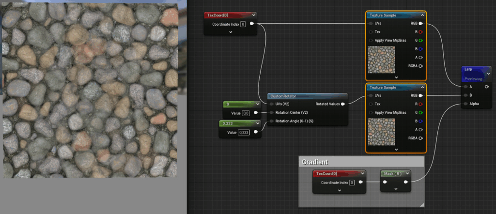
Now let’s try the same with applied dithering on the weights: In this example, a texture is sampled with two different coordinates and the results are then blended.

Now, just for the sake of it, this happens when you just blend the coordinates instead of the textures and then sample the texture once:

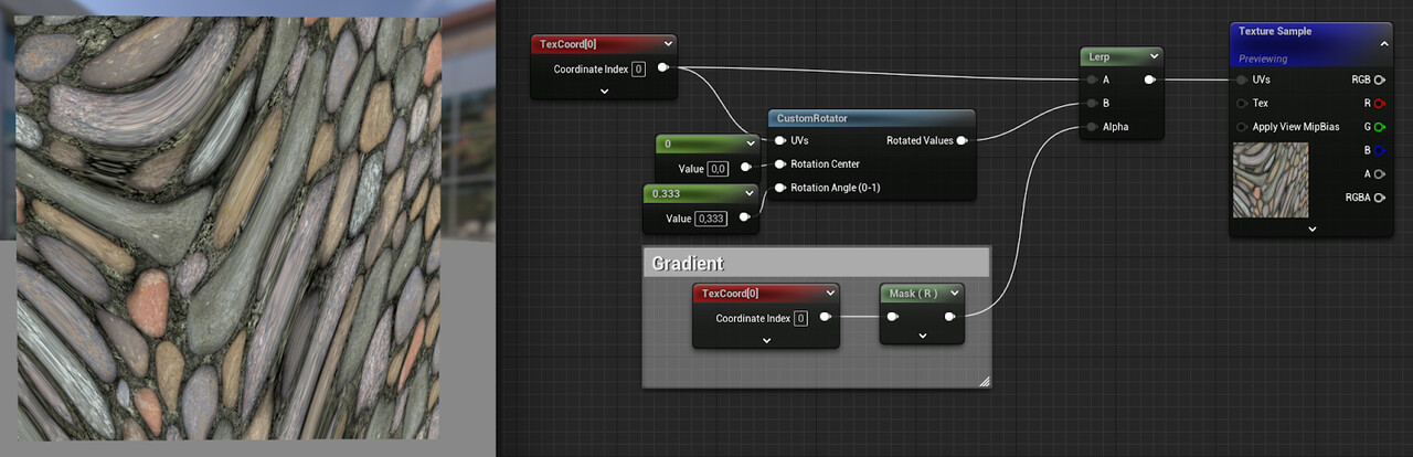
Obiously, blending UVs doesn’t make sense, but let’s what happens when we use dithering to use only one of the two UVs per pixel:

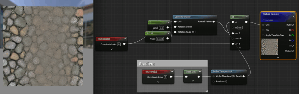
Better, I guess? It already resembles the blended textures, but the transition looks ugly. The reason for that is the mip-map calculation. When sampling a texture, the mip-map to use is calculated by looking at the difference between the coordinates of the current pixel and the coordinates of the previous pixel. The bigger this difference, also called derivative, the smaller the resolution of the mip-map to be used.
But due to the dithering, the coordinates of the previous pixel are completely unrelated and way off, so the texture is sampled as if it were far away from the camera, using a mip map with a lower resolution.
With mip-mapping disabled, the transition area is cleaned up:

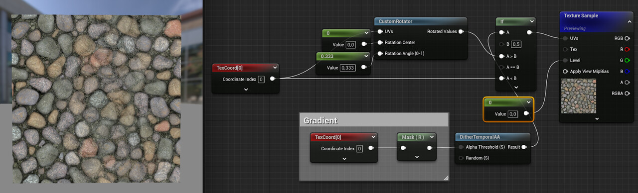
That’s not the actual solution to this problem, though. Mip maps exist for a reason (multiple ones, to be exact). Without mip-mapping, the texture can’t be streamed in, and is loaded at full resolution.
And if you don’t care about memory usage, sampling the texture at full resolution even in the distance won’t look great, as shimmering is introduced.
Thankfully, you don’t need to rely on the automatic derivative calculation, you can also specify them manually. In the example below, the derivatives for one of the coordinate sets are calculated and then used throughout:

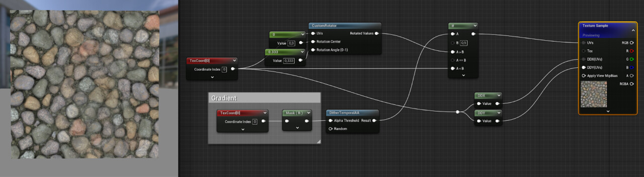
This works because even though the second UVs are rotated differently, the scale remains the same, so even if the derivatives differ slightly, most of the time the same mip-map is going to be used.
Now let’s rotate the derivatives as well:

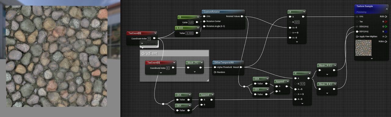
The visual difference isn’t noticeable in this case, but with flatter viewing angles, not rotating the derivatives together with the coordinates can make a difference. But then again, using dithering instead of actual blending is already a far bigger compromise, so I don’t feel bad about skipping this step.

Building the hex tiling material

Setting up the coordinates

After having looked up other implementations of hex tiling, I started building my version using dithered UVs.
The first step is to create three separate layers with coordinates:

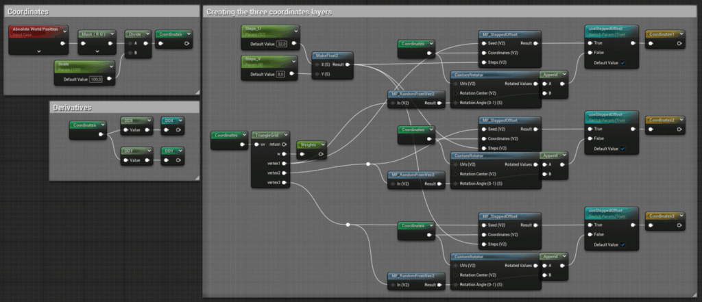
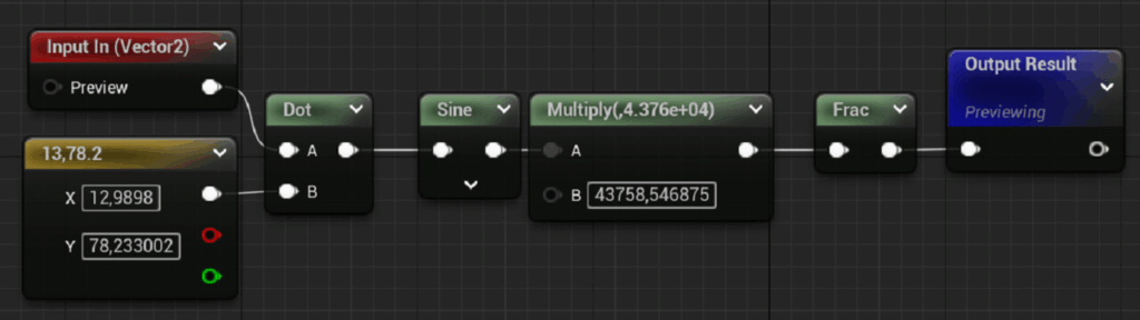
The TriangleGrid node contains custom hlsl code borrowed from Thomas Deliot and Eric Heitz:

// Scaling of the input
uv *= 3.464; // 2 * sqrt (3)
// Skew input space into simplex triangle grid
const float2x2 gridToSkewedGrid = {1.0, 0.0, -0.57735027, 1.15470054};
float2 skewedCoord = mul(gridToSkewedGrid, uv);
// Compute local triangle vertex IDs and local barycentric coordinates
int2 baseId = int2(floor(skewedCoord));
float3 temp = float3(frac(skewedCoord), 0);
temp.z = 1.0 - temp.x - temp.y;
if (temp.z > 0.0)
{
    w = temp.zyx;
    vertex1 = baseId;
    vertex2 = baseId + int2(0, 1);
    vertex3 = baseId + int2(1, 0);
}
else
{
    w = float3(-temp.z, 1.0 - temp.y, 1.0 - temp.x);
    vertex1 = baseId + int2(1, 1);
    vertex2 = baseId + int2(1, 0);
    vertex3 = baseId + int2(0, 1);
}
return 1.0f;

I recommend reading the paper to get a better understanding of what this code does. The most important thing to understand is that while the technique is called hex tiling, the shapes that are blended together aren’t hexagons, but the adjacent triangles that make up each hex tile

The node returns:

• a float3 containing the weights of the triangles
• three float2s containing index values of the hexagon containing the current triangle.

The hexagon IDs are subsequently used to compute random values for the tiles:

These values are then employed as angles to rotate the coordinates. Afterwards, the angles are appended to the coordinates, since you’ll need them later on.
As you can see, in my material graph, there is an alternative to rotating the coordinates, called stepped offsets.

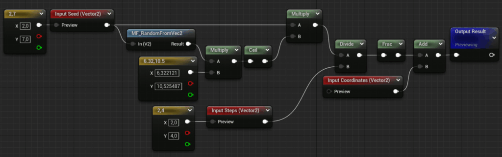
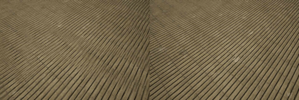
Stepped Offsets

Rotating the coordinates works very well for chaotic, directionless surfaces like grass, dirt or concrete. But as soon as a texture has a noticeable orientation (like wood grain), randomly rotating the tiles will break it. Therefore, I added the option to just shift the coordinates instead. And since there are many cases where textures contain grid-like structures, the offset is applied in discrete. For instance, if your texture consists of 10×10 plates, you can set the Steps_U and Steps_V parameters accordingly so that the UVs are only offset in 0.1 steps, ensuring that the gaps between the plates still align with each other.

This is the Stepped Offsets material function:

Below you see a comparison between stepped offsets on the right and non-stepped offsets on the left:

Combining the Coordinates

Now that we have the coordinates, let’s combine them:

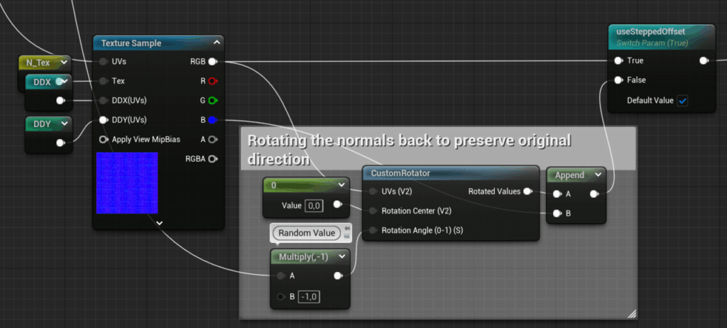
The combined coordinates are then used to sample the textures. Remember to use derivatives that are calculated using the original coordinates before the offsets or rotations were applied!

Another important detail: Whenever you rotate UVs, make sure to rotate the normals accordingly the other way around, otherwise they’ll point in the wrong direction. That’s the reason why the angles were appended to the coordinates earlier.

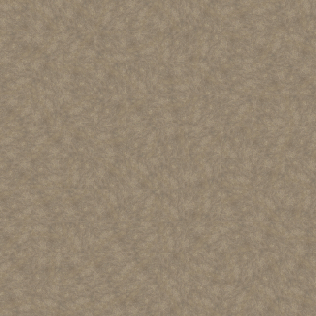
The Results

Here is a comparison of classic tiling, hex tiling with random stepped offsets and with random rotations.

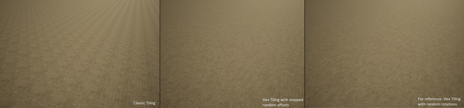
Since the texture doesn’t have that much contrast, dithering works very well in this case, but your mileage may vary. The focus of this implementation was versatility (hence the option for stepped offsets) and speed (hence the dithering instead of sampling the texture multiple times).

It has its limitations though if it comes to quality. I wouldn’t recommend adding parallax mapping for example, since it will break in the transition areas. Still, if you’ve read this article up to this point, I’m hoping I could provide you with some helpful insights that will turn out to be helpful. If you come up with any changes or improvements to this implementation I’d be happy to know about them!